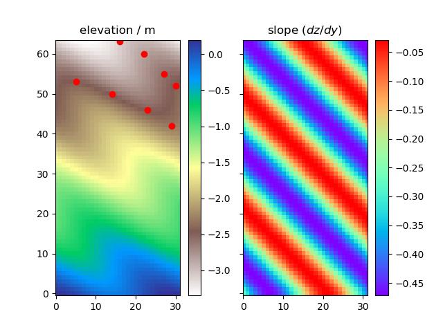
Figure 4.1: Contour plots of elevation (left) and slope (right). Feature markers are shown as red disks.
Next: GNU Free Documentation License, Previous: Boundary Definition File, Up: Top [Contents][Index]
Examples of input files that demonstrate how to use FullSWOF-utils programs are included in the demo directory. Sample height data, in the file topography.txt, is also provided.
To run the demos directly, first change the current working directory to the demo directory. Then execute the individual program (see Usage for the command line syntax).
The input files for makeBoundary may be viewed with a text
editor. To experiment with the control parameters, first back up the
distributed input files and then edit the parameter values as desired.
Note that the makeBoundary program will overwrite its output
file if it already exists.
Running slope.py provides an opportunity to test the effect of
marker positioning. Contour plots of elevation and slope are displayed
when the m key is pressed. The elevation contour plot allows the
feature of interest to be identified. Markers are placed in pairs on
either side of the channel feature. An example of a set of marker pairs
is shown in Figure 4.1.

Figure 4.1: Contour plots of elevation (left) and slope (right). Feature markers are shown as red disks.
slope.py draws a straight line between each pair of markers.
A search procedure reveals the position along each line at which the
elevation is a minimum. The set of minumum positions identifies the
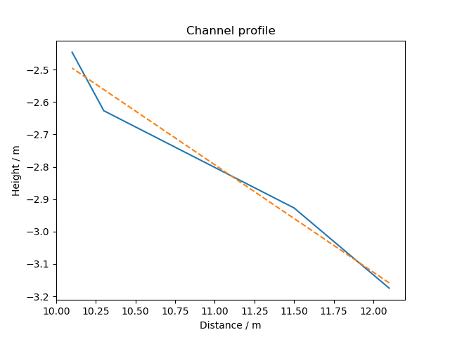
centre-line of the channel. The profile of the channel is plotted and
displayed when the p key is pressed. The profile calculated from
the example set of marker pairs is shown in Figure 4.2.

Figure 4.2: Elevation plotted against distance from bottom boundary.
The blue line in Figure 4.2 shows the height variation of the channel centre-line. The best-fit line is shown by the dashed red line. The gradient of the best-fit line and the intercept on the y-axis are printed to standard output. The data points that define the blue line are written to the file 1D.txt when the s key is pressed. The file is overwritten if it already exists.
Next: GNU Free Documentation License, Previous: Boundary Definition File, Up: Top [Contents][Index]